Experimental exploration of cavity flow physics
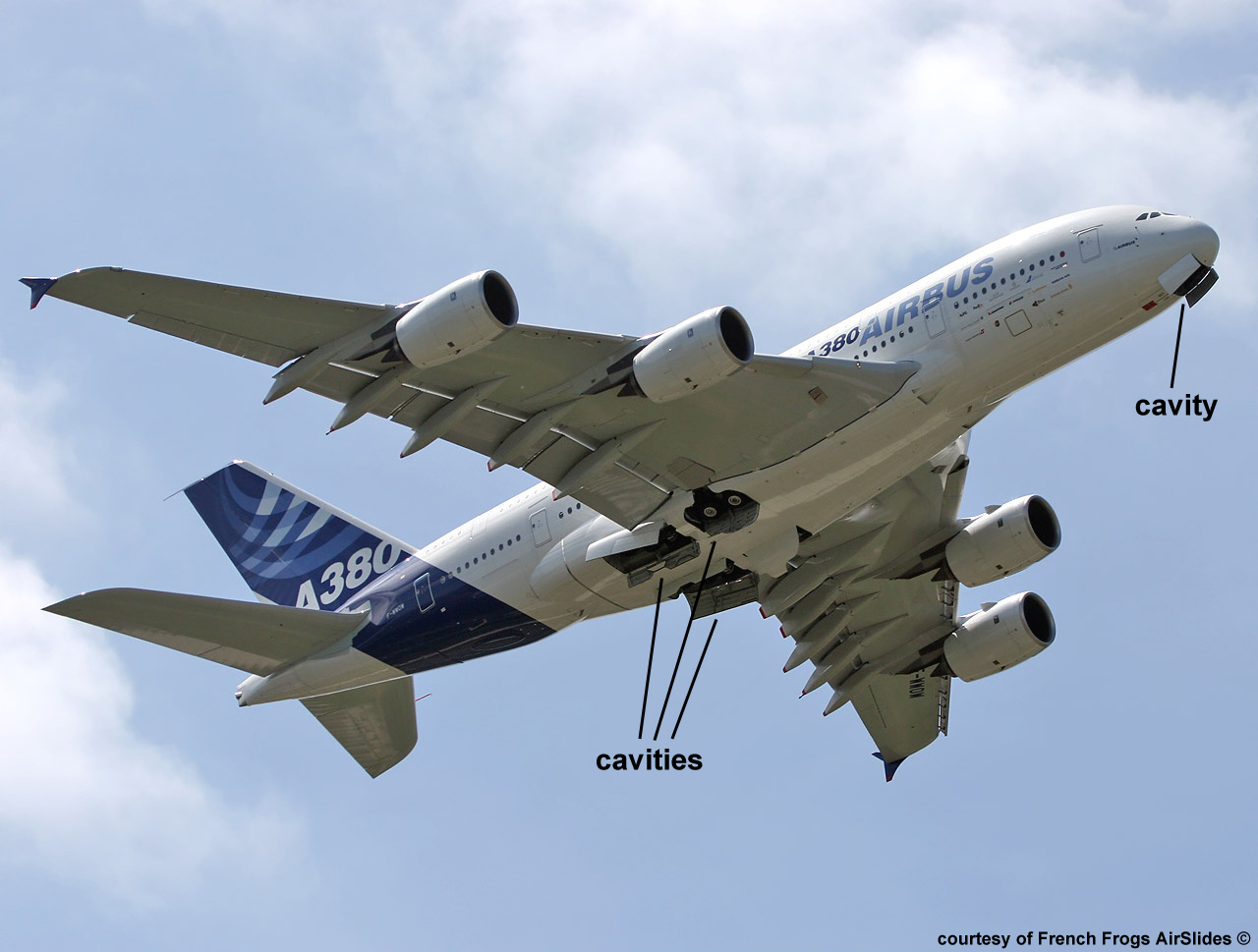
The acoustic resonance of a flow over a cavity is a problem experienced in several practical situations. For instance, one can hear some very strong, drum-like pusating noise inside a car that moves at 40 or more miles per hour with the rear windows lowered. Another example is the vibration felt inside an aircraft that extends the weels before landing, Fig. 1. |
|
| Figure 1: An example of cavity flow noise: the open bays of an aircraft landing gear. |
Figure 2 below explains what happens in these cases. The air flowing over an opening (the cavity) in the vehicle body (like the open window of a car or the landing gear bays of an aircraft) creates some air vortices. These vortices (green in the figure) travel with the flow stream until they reach and impact the other end (point B) of the opening thus creating strong acoustic waves (i.e. noise, red) that propagates in the environment. These waves reach the beginning of the cavity (point A) where they stimulate the formation of new vortices that will repeat the process thus creating even more noise. Therefore the phenomenon is continually reinforcing itself until a condition is quickly reached where a very strong pulsating noise is produced, as in the examples above. The pulsations occur at discrete frequencies that depend on the velocity of the air (i.e. the velocity of the vehicle) and on the size of the cavity. |
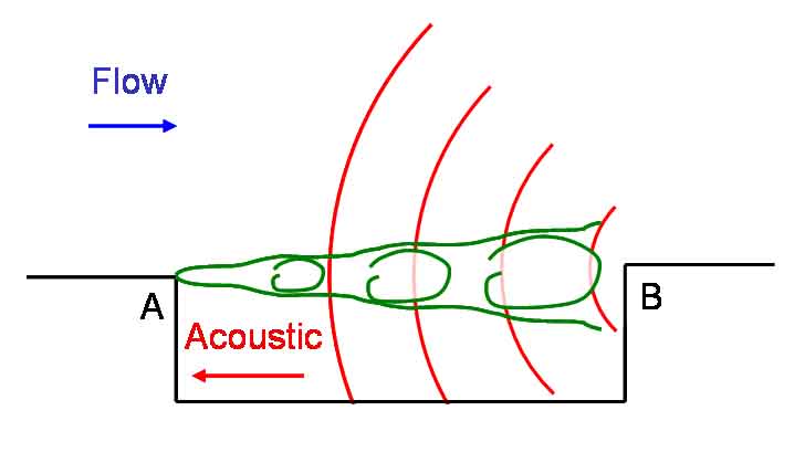 |
| Figure 2: The mechanism of cavity flow resonance. |
Several techniques can be used to avois this pulsations. For instance cars with a roof hutch use a small spoiler that deviates the vortices above the hutch (the cavity) such that they do not impact its rear end. This spoiler actually creates some aerodynamic resistance but this is not high since cars travel at relatively low speeds. Aicraft usually travel at higher speeds where a spoiler may not work well and thus smarter solution are sought. |
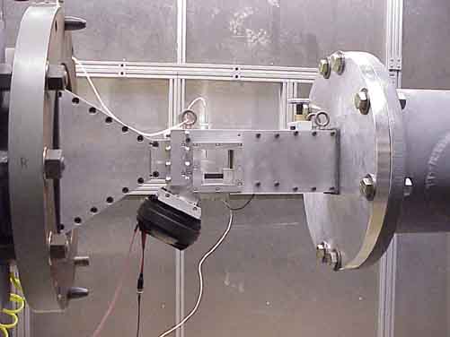
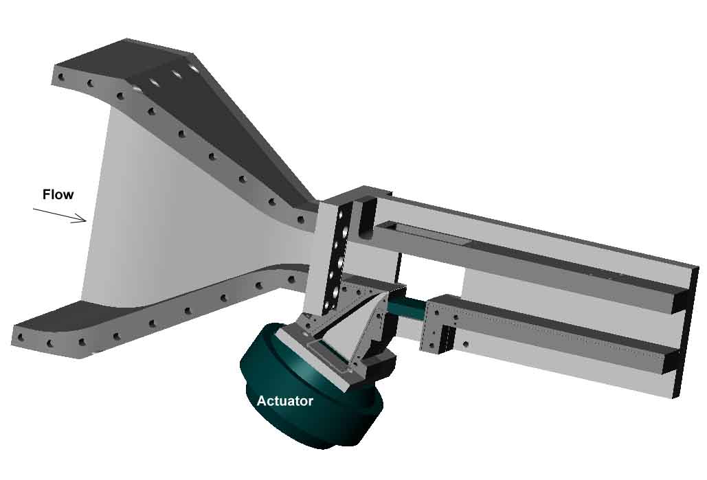
In order to develop better techniques to reduce cavity flow resonance it is important to study and to understand its physics. To this aim I designed a small wind tunnel in The Ohio State University which has a cavity recessed in the floor, Figs. 3 and 4. The wind tunnel can operate continuously in the subsonic range and has a modular construction that allows different acoustic and optical measurements to study what happens in the test section (a more in depth description of the experimental apparatus is available in my publications). In Cranfield University I am using a similar facility to explore the acoustics of cavities incorporating internal diaphragms for disrupting the self-reinforcing phenomenon described in Fig. 1. These measurements will complement and complete other studies on cavity-flow and on the control of its resonant noise. |
 |
 | |
| Figure 3: Picture of the OSU-GDTL cavity flow facility. |
Figure 4: 3D section drawing of the OSU-GDTL cavity-flow facility. |
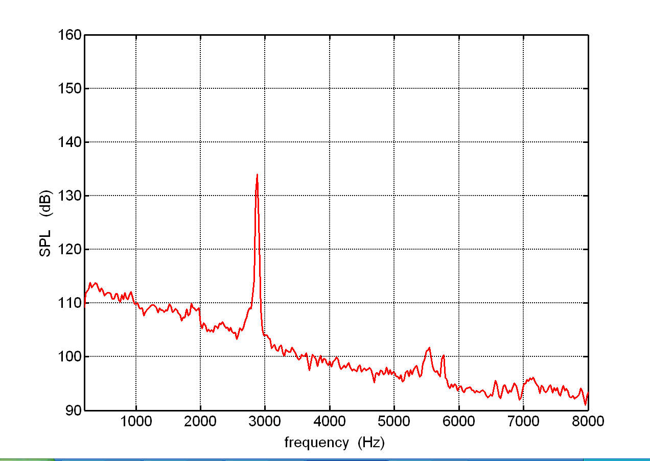
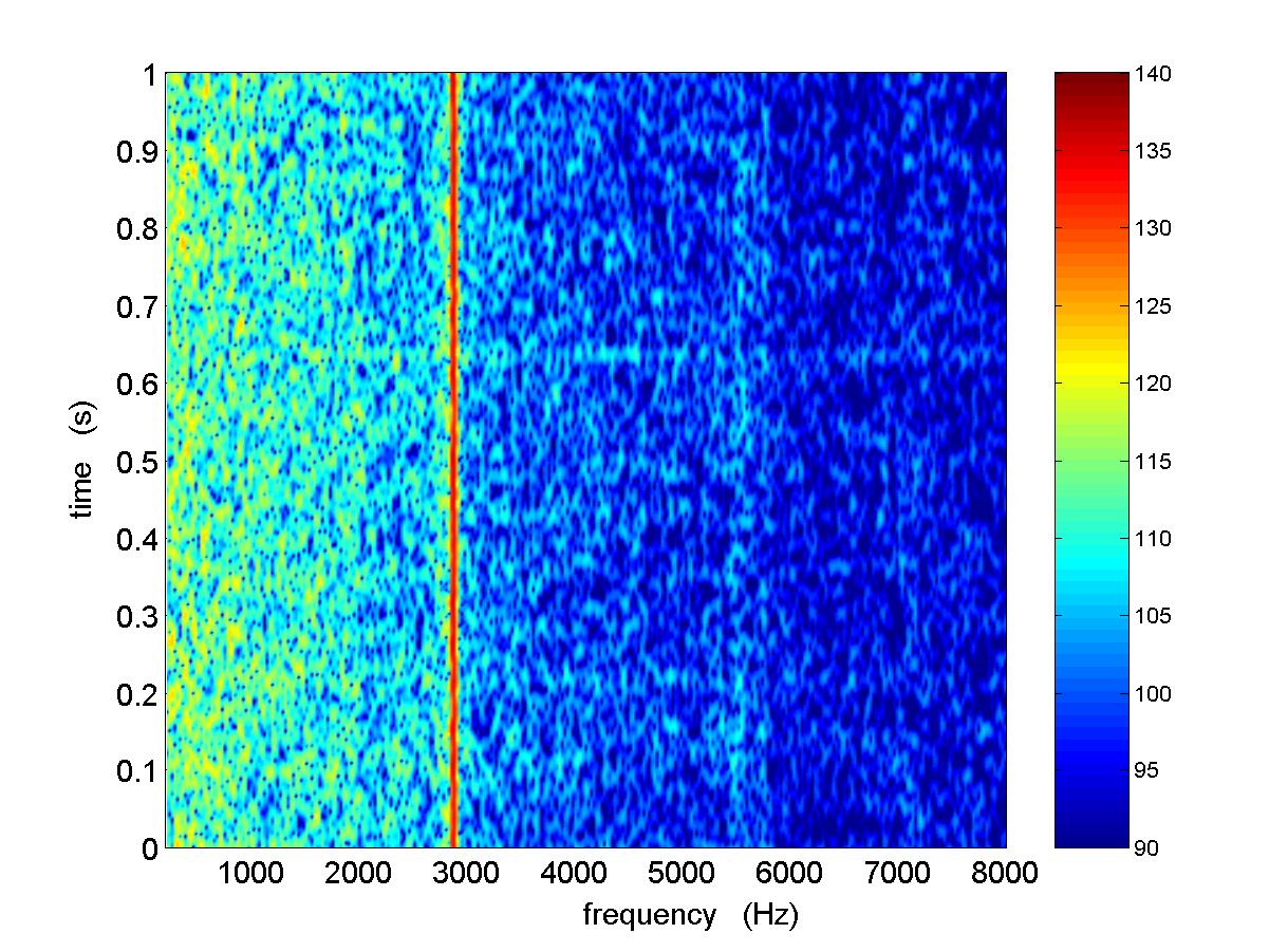
Typically, dynamic pressure transducers (tiny microphones) are used to measure the nature and the evolution of the noise in different locations of the test section. For instance, Fig. 5 shows the acoustic spectrum measured at Mach 0.3 (about 220 mph) by a transducer placed in the middle of the floor of the cavity setup in Figs. 3 and 4. The peak at the frequency of about 2850 Hz represents the intense pulsating cavity flow noise. The noise at this frequency remains strong and steady in time as evidenced by the continuous red line in the spectrogram in Fig. 6 where color is used to express the intensity of the noise in dB: the darker the red, the stronger the noise. This behavior can be observed in some velocity ranges and is called single-peak resonance. |
 |
 | |
| Figure 5: Noise spectrum of Mach 0.30 flow. |
Figure 6: Spectrogram of Mach 0.30 flow. |
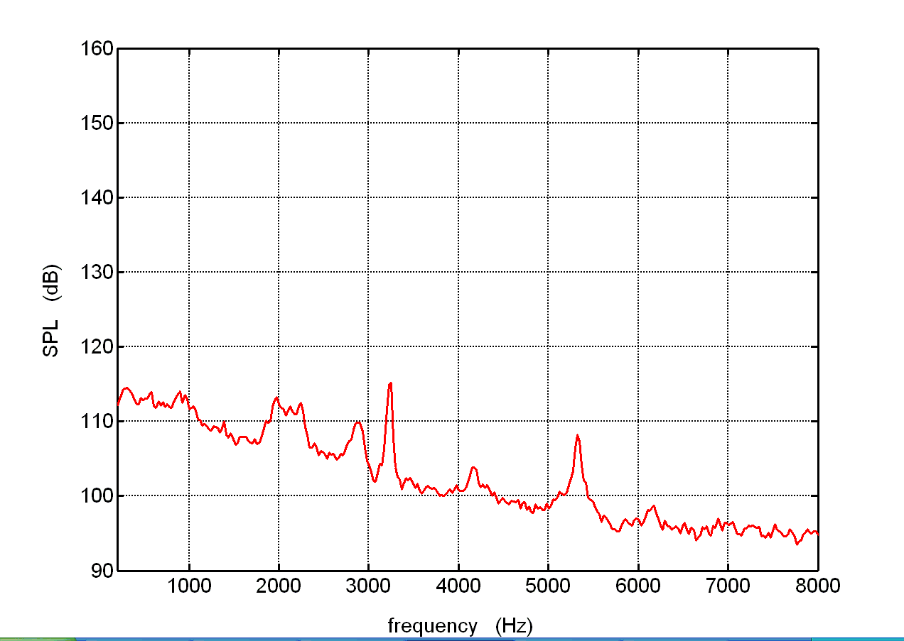
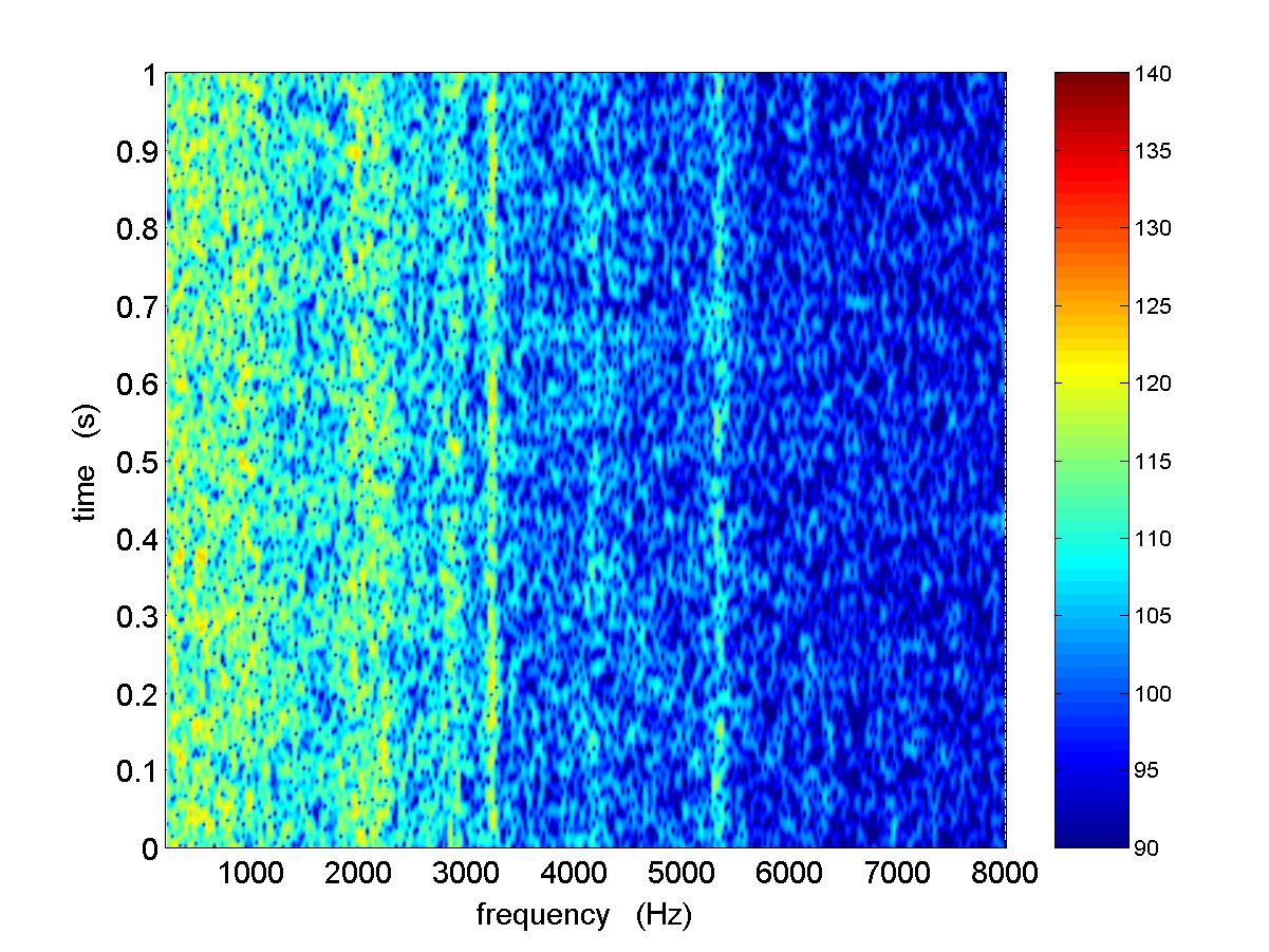
At other velocities the behavior is quite different. For instance, Figure 7 shows that the acoustic spectrum measured at Mach 0.32 (about 250 mph) has several smaller peaks (multi-peak resonance). Furthermore, as visible in the spectrogram of Fig. 8, these peaks do not remain steady in time and rapid switching occurs between them. This switching produces a less efficient cavity resonance since no single peak locks-in to dominate the spectrum. I produced a similar switching with open-loop and closed-loop control techniques and used it to reduce strong single-peak resonance (AIAA 2004-2123). |
 |
 | |
| Figure 7: Noise spectrum of Mach 0.32 flow. |
Figure 8: Spectrogram of Mach 0.32 flow. |
Figures similar to 5 and 7 were obtained at other Mach numbers from 0.2 to 0.7 (i.e. from about 150 to 520 mph). Figure 9 summarizes these measurements; on the horizontal axis is the frequency, on the vertical axis is the Mach number (the flow velocity). Similar to Figs. 6 and 8, color is used to express the intensity of the noise in dB. Superimposed to this figure are also the lines R1, R2, R3, and R4 of the 1st, 2nd, 3rd, and 4th modes predicted by the model of Rossiter (continuous white lines), the line L1 of the 1st longitudinal standing wave, and the lines T1 and T2 of the 1st and 2nd transversal standing waves (dotted white lines). The latter are caused by the walls and ceiling of the wind tunnel. Figures 5 and 7 are basically "horizontal slices" of Fig. 9 taken at Mach 0.3 and 0.32, respectively. By comparing Figs. 5 and 9 it is clear that the strong peak of Fig. 5 corresponds to the 3rd Rossiter mode. |
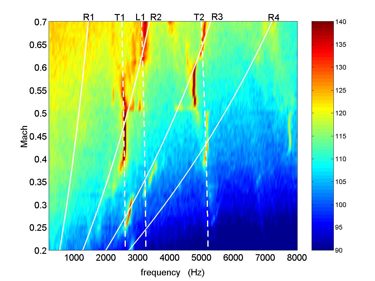 |
| Figure 9: Noise frequency and intensity (dB) for flow between Mach 0.2 and 0.7 . |
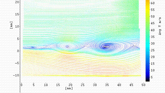
The arrays of transducers for noise measurement are used in conjunction with qualitative flow visualizations, Fig. 10, and with the data obtained using 2D Particle Image Velocimetry, Fig. 11. |
 |
 | |
| Figure 10: Instantaneous image of Mach 0.30 flow with smoke in cavity floor. |
Figure 11: Streamlines of Mach 0.30 flow relative to a reference frame moving with the speed of the vortices. |
The images can be phase-locked to the shedding frequency of the shear-layer vortices or to the forcing signal of the actuator used for control. Both instantaneous and phase-averaged images are obtained in an effort to identify variations between baseline (non-controlled) and controlled cases. The results obtained show that the behavior of the vortices spanning the cavity matches the empirical predictions given in classical literature. Reduction of the acoustic resonance with control is accompanied by subtle changes in the flow structure and behavior as evidenced by comparing Fig. 12 with Fig. 11 (see also Fig. 1 in the section on cavity flow control). |
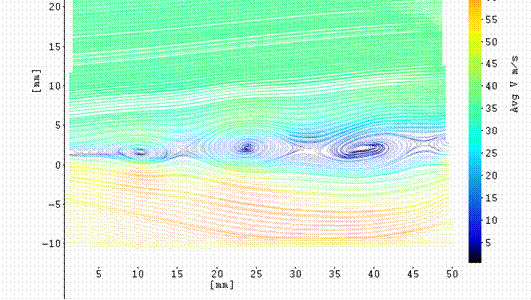 |
| Figure 12: Streamlines of Mach 0.30 flow with actuation at 3250 Hz relative to a reference frame moving with the speed of the vortices. |
The detailed results obtained with these techniques are being complemented by schlieren images and hot-wire velocity measurements, and will be analyzed and matched against the most recent models of cavity flow. |
Additional information on this research can be found in:
|
| MD current research | MD research | MD home |